Groundwater Flow Modeling - Methods
Types of Groundwater Models
A model of any natural system is a simplified representation of that system. Groundwater models incorporate parts of the hydrologic cycle that effect groundwater. Figure 1 shows a conceptual model of a local hydrologic system that can be modeled. The system includes natural processes such as recharge from precipitation, evapotranspiration from non-cultivated vegetation, and the exchange of flow between groundwater and streams. Models also include anthropogenic processes like pumping wells, irrigation, artificial recharge ponds, and controlled surface water flows using dams or sluice gates.
A groundwater model is a mathematical representation of a groundwater flow system. There are three main types of groundwater models:
Simple Mathematical models
Analytical Models, and
Numerical Models

Figure 1: Example of a conceptual model (adapted from USGS)
A simple mathematical model can be used to represent a characteristic of a groundwater system such as the groundwater elevation in an area. Figure 2 shows five locations where the groundwater level elevation is known. The average groundwater level (1321.5 ft) is one example of a simple model that can be used to estimate the water level in the area.
An analytical model is a more complicated mathematical function that describes the relationship between processes. A fundamental analytical model used by groundwater scientists is the Theis equation, which calculates the flow of heat or water. In groundwater studies, this equation calculates the amount of drawdown expected at any distance from a pumping well over time. Figure 3 is an example of a Theis solution at 1, 10, and 50 years of pumping within three miles from the pumping well.
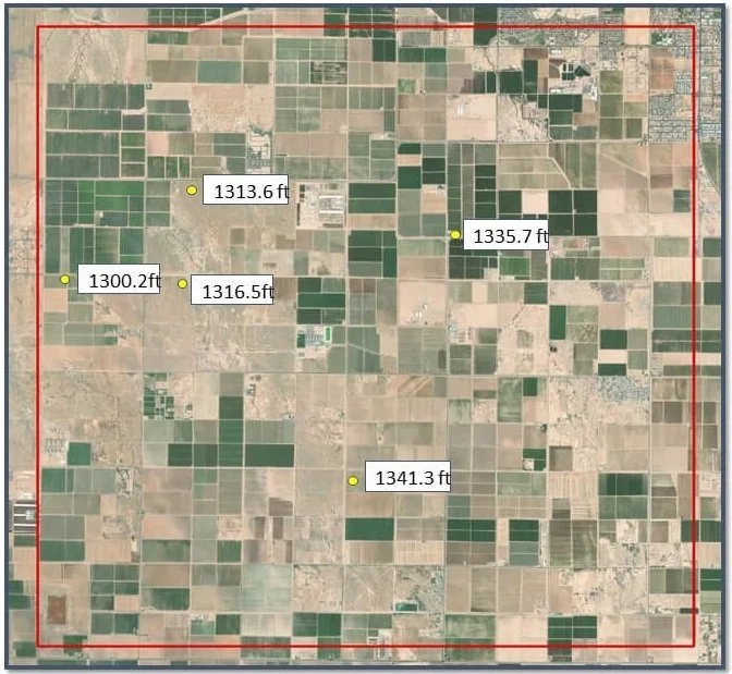
Figure 2: Example of a simple mathematical model
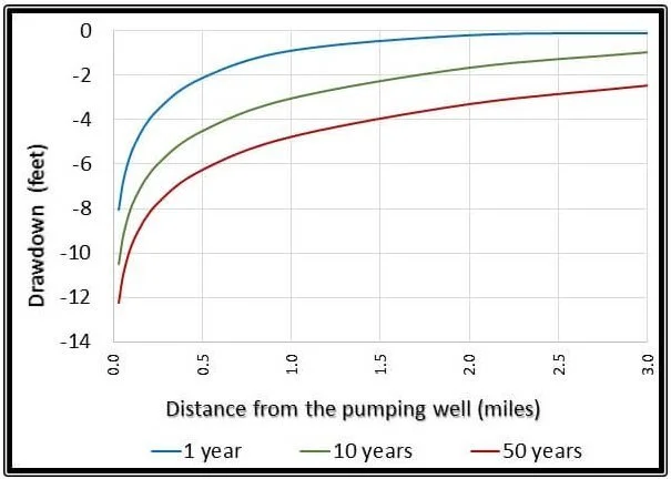
Figure 3: Example of drawdown at a well with distance and time calculated using the Theis Equation
Analytical solutions are based on assumptions about the system to which they apply. For example, the Theis equation assumes:
1. Confined conditions,
2. The well fully penetrates the aquifer,
3. Aquifer thickness is uniform,
4. Hydraulic properties are uniform,
5. The aquifer is of infinite extent, and
6. Pumping is a constant rate.
These assumptions limit the use of the Theis equation and make it inappropriate in some situations. However, there are hundreds of analytical models (including modifications to Theis’ equation) that can be applied to groundwater systems (HydroSolv, Inc., 2002).
Numerical models are used for complex groundwater systems that are difficult or impossible to be adequately described by simple mathematical or analytical solutions. For example, they can accommodate the complexity of a system depicted in Figure 1, with conditions that vary over time. Unlike analytical solutions that can be solved for any location in the model, numerical models rely on solving equations between two or more distinct and adjacent locations.

Figure 4: Example of a three-dimensional block-centered finite-difference grid (Harbaugh 1989)
One example of a numerical model is a finite-difference model using a block, or grid cell structure (Figure 4). The groundwater flow equation is solved at the center of each grid cell by a linear function. This allows some processes which are non-linear to be incorporated into the linear equations, thus an approximate solution can be obtained.
Therefore, the groundwater practitioner, “Goldilocks,” must approach each problem with an eye toward the best solution to groundwater modeling that is: not too simple, leaving out important processes (too little); not overly complex, requiring too much detail (too much); but is just complex enough to provide a useful answer (just right) (Figure 5).

Figure 5: Goldilock’s question
For more in-depth information, LWS has a blog series on “Numerical Groundwater Flow Modeling,” check it out HERE!
If you have any water resources issues, LWS can help; please contact us for help
Maura Metheny, Ph.D., P.G. maura@lytlewater.com
Bruce Lytle, P.E. bruce@lytlewater.com
Anna Elgqvist, EI anna@lytlewater.com
Marlena McConville marlena@lytlewater.com
References:
Harbaugh, A.W., and McDonald, M.G., 1996. User's documentation for MODFLOW-96, an update to the U.S. Geological Survey modular finite-difference ground-water flow model. U.S. Geological Survey Open File Report 96-485. Available at https://pubs.usgs.gov/of/1996/0485/report.pdf.
HydroSolv, Inc., 2002. AquteSolv for Windows, User‘s Guide. Reston Virgina. Available at http://www.aqtesolv.com/.
Theis, C.V., 1935. The relation between the lowering of the piezometric surface and the rate and duration of discharge of a well using groundwater storage, Am. Geophys. Union Trans., vol. 16, pp. 519-524